
David Anderson
Originally written in June 1999
The beauty of the blending function as it applies to projecting geodesic patches is that any smooth function with a value of zero on the edges can be used.
 In the previous paper, Connecting Superprojected and Subprojected Geodesic Patches, the blending function was developed as the normalized product of three simple distance components: each was the respective perpendicular distance of an unprojected vertex from an unprojected edge of the geodesic patch.
This composite blending function was used to seamlessly combine patches with different projection parameters.
In the previous paper, Connecting Superprojected and Subprojected Geodesic Patches, the blending function was developed as the normalized product of three simple distance components: each was the respective perpendicular distance of an unprojected vertex from an unprojected edge of the geodesic patch.
This composite blending function was used to seamlessly combine patches with different projection parameters.
The simple blending function causes the shape of the patch to change smoothly across its surface, and yet keep its edges untransformed. Edges of patches with different projection paramters align, and may be joined together in the same structure without a seam. Unfortunately, the simple blending function is otherwise uninteresting. Although the product of three variables, it simply changes smoothly and uniformally, at least from the edge of the patch to its center.
Edge distance is a perfectly good component blending function, of course, but it is effectively only a simple identity function: b(x) = x, where x is the perpendicular distance of the vertex from the edge. The essential properties of the component blending function are that it is continuous across the surface of the patch, and that it's value is 0 on the edge. The simple distance function satisfies these requirements, but there are other component blending functions which can produce more interesting results.
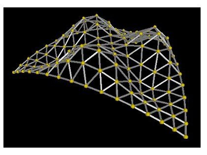 For example, the 15-frequency icoshedral patch pictured on the left has a component blending function b(x) = x2-x3, where x again is the perpendicular distance of the vertex from the edge.
Instead of a simple smooth curve, we now see hills and valleys.
Click here for a vrml model of the patch.
Though the component blending function is a only a polynomial, when it is used in the composite blending function, effectively multiplied by itself after being rotated equilaterally - mixing with itself at 120o and 240o - a more complex landscape emerges.
For example, the 15-frequency icoshedral patch pictured on the left has a component blending function b(x) = x2-x3, where x again is the perpendicular distance of the vertex from the edge.
Instead of a simple smooth curve, we now see hills and valleys.
Click here for a vrml model of the patch.
Though the component blending function is a only a polynomial, when it is used in the composite blending function, effectively multiplied by itself after being rotated equilaterally - mixing with itself at 120o and 240o - a more complex landscape emerges.
Polynomials are especially nice component blending functions because of all the different curves that can arise: most any function can be approximated using a polynomial of a high enough degree. However, the higher the degree, the more the error in the polynomial increases, so other functions may also be useful to a surface designer. A transcendental function could be used: for instance, b(x) = sin(x) is a function that meets the blending component requirements. A shifted logarithmic function also qualifies: b(x) = ln(x+1) will work when x > -1. In fact, there are many other functions that fit the requirements - each potentially gives a new, interesting shape to the patch.
It also must be noted that the same component blending functions need not be used for each equilateral direction. Using different component blending functions in the different directions will generally lead to assymetrically-shaped surfaces. This may be very important if determining a surface that will surround an irregular volume is required. However, these patches will still be able to be mated with their adjoining neighbors since the position of the edges is not modified by the projection.
One of the important emergent properties of component blending functions is that since the values are continuous and the edge boundary condition is set up the way it is, then if b1(x) and b2(x) are component blending functions, then so is b1(b2(x)). This implies that polynomials, transcendentals, and other qualifying component blending functions may be convolved without any problems.
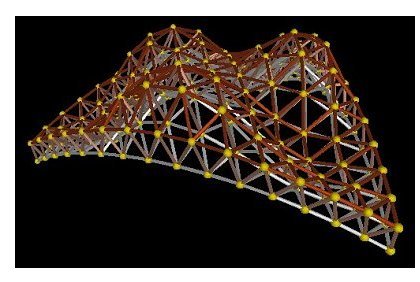 Of course, just because we now have a means to generate geodesic patches with irregular surfaces doesn't mean we have to sacrifice structural strength.
The patch pictured on the right has the same mathematical structure as the previous patch, but also includes an external warped octet truss to keep it rigid.
This truss follows the contour of the smooth hills and valleys of the patch, and it's hieght varies directly with it's projected distance.
Of course, just because we now have a means to generate geodesic patches with irregular surfaces doesn't mean we have to sacrifice structural strength.
The patch pictured on the right has the same mathematical structure as the previous patch, but also includes an external warped octet truss to keep it rigid.
This truss follows the contour of the smooth hills and valleys of the patch, and it's hieght varies directly with it's projected distance.
The truss can be internal or external; it is based on the same principals that were used for it's development in Planning a Bigger Dome, Part II. In these bumpy-patches, the deformation of the constituent octahedron/tetrahedron matrix is locally regular, despite being relatively irregular globally. As the frequency of the patch increases, it becomes smoother locally, and the truss system is not projected as far away from the surface. In the limit, where the frequency of the geodesic becomes infinite, the patch and truss become one, a solid surface.
At this point, the rest of the exploration is empirical. Different component blending functions may give very different results, and the resulting surfaces may have applications in many different areas. Cataloging the composite blending functions would be an entertaining mathematical endeavor, and would lead to a tremendous repositiory of design information.